Sparse Matrices For Efficient Machine Learning

Introduction

Sparse matrices are common in machine learning. While they occur naturally in some data collection processes, more often they arise when applying certain data transformation techniques like:

• One-hot encoding
• CountVectorizing
• TfidfVectorizing

Let’s step back for a second. Just what the heck is a sparse matrix and how is it different than other matrices?

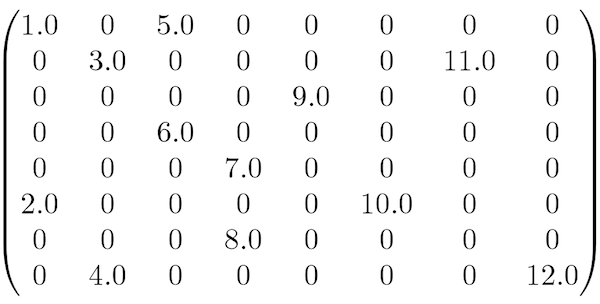
Turns out there are two major types of matrices: dense and sparse. Sparse matrices have lots of zero values. Dense matrices do not.

Here is an example of a sparse matrix:

Because sparse matrices have lots of zero values, we can apply special algorithms that will do two important things:

1. compress the memory footprint of our matrix object
2. speed up many machine learning routines

Since storing all those zero values is a waste, we can apply data compression techniques to minimize the amount of data we need to store. That is not the only benefit, however. Users of sklearn will note that all native machine learning algorithms require data matrices to be in-memory. Said another way, the machine learning process breaks down when a data matrix (usually called a dataframe) does not fit into RAM. One of the perks of converting a dense data matrix to sparse is that in many cases it is possible to compress it so that it can fit in RAM.

Additionally, consider multiplying a sparse matrix by a dense matrix. Even though the sparse matrix has many zeros, and zero times anything is always zero, the standard approach requires this pointless operation nonetheless. The result is slowed processing time. It is much more efficient to operate only on elements that will return nonzero values. Therefore, any algorithm that applies some basic mathematical computation like multiplication can benefit from a sparse matrix implementation.

Sklearn has many algorithms that accept sparse matrices. The way to know is by checking the fit attribute in the documentation. Look for this: X: {array-like, sparse matrix}.

At the time of this writing, the following sklearn 0.18.1 algorithms accept sparse matrices:

Classification

• Logistic Regression
• SGDClassifier
• Perceptron
• PassiveAggressiveClassifier
• NuSVC
• LinearSVC
• SVC
• KNeighborsClassifier
• RadiusNeighborsClassifier
• NearestCentroid
• MultinomialNB
• BernoulliNB
• DecisionTreeClassifier
• BaggingClassifier
• RandomForestClassifier
• ExtraTreesClassifier
• AdaBoostClassifier
• VotingClassifier
• OneVsRestClassifier
• OneVsOneClassifier
• OutputCodeClassifier
• MultiOutputClassifier
• MLPClassifier

Regression

• Linear Regression
• Ridge Regression
• Lasso Regression
• ElasticNet
• SGDRegressor
• PassiveAggressiveRegressor
• RANSACRegressor
• KernelRidge
• SVR
• NuSVR
• LinearSVR
• KNeighborsRegressor
• RadiusNeighborsRegressor
• DecisionTreeRegressor
• BaggingRegressor
• RandomForestRegressor
• ExtraTreesRegressor
• AdaBoostRegressor
• MultiOutputRegressor
• MLPRegressor

Clustering

• KMeans
• MiniBatchKMeans
• SpectralClustering
• DBSCAN
• Birch

Decomposition

• TruncatedSVD
• NonnegativeMatrixFactorization
• LatentDirichletAllocation

Feature Selection

• VarianceThreshold
• RecursiveFeatureElimination

Other

• OneClassSVM
• NearestNeighbors
• LSHForest
• RandomTreesEmbedding

Applications & Workflow

I will cover several interesting topics in this section. First, there is a great tool called spy(). It is available in the Matplotlib library and it allows us to visually inspect a matrix for sparsity. Next, Scipy has the Compressed Sparse Row (CSR) algorithm which converts a dense matrix to a sparse matrix, allowing us to significantly compress our example data. And finally, I will run three classification algorithms on both dense and sparse versions of the same data to show how sparsity leads to markedly faster computation times.

Setup

I generated a sparse 2,000 by 10,000 dataset matrix composed of zeros and ones.

import numpy as np
np.random.seed(seed=12)  ## for reproducibility
dataset = np.random.binomial(1, 0.1, 20000000).reshape(2000,10000)  ## dummy data
y = np.random.binomial(1, 0.5, 2000)  ## dummy target variable

Spy()

I mentioned Matplotlib’s spy() method which allows us to visualize the sparsity of a dataset.

Note: the %matplotlib inline is for Jupyter notebook users. Feel free to omit it otherwise.

%matplotlib inline
import matplotlib.pyplot as plt
plt.spy(dataset)
plt.title("Sparse Matrix");

Notice that the graph is mostly white. For comparison purposes, here’s a dense matrix.

np.random.seed(seed=43)
plt.figure(figsize=(14,12))
plt.spy(np.random.binomial(1, 0.9, 20000000).reshape(2000,10000))
plt.title("Dense Matrix");

Scipy CSR

We have a data matrix called dataset. We already know it is very sparse so let’s go ahead and transform it with Scipy’s CSR.

from scipy.sparse import csr_matrix
sparse_dataset = csr_matrix(dataset)

Compression

import seaborn as sns

dense_size = np.array(dataset).nbytes/1e6
sparse_size = (sparse_dataset.data.nbytes + sparse_dataset.indptr.nbytes + sparse_dataset.indices.nbytes)/1e6

sns.barplot(['DENSE', 'SPARSE'], [dense_size, sparse_size])
plt.ylabel('MB')
plt.title('Compression')

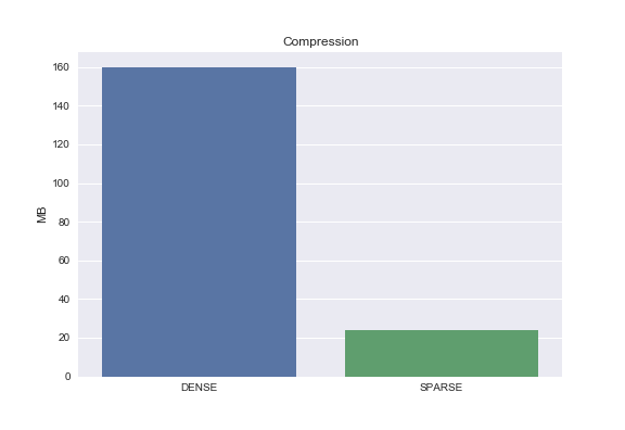
From the graph above we can see that the dense matrix is 160 MB while the sparse matrix is 24 MB. That’s 85% compression! Granted we started with a pretty sparse matrix.

Computation Time

I ran three different classification algorithms - Bernoulli Naive Bayes, Logistic Regression, Support Vector Machines - and checked processing times for each.

from sklearn.naive_bayes import BernoulliNB
nb = BernoulliNB(binarize=None)
%timeit nb.fit(dataset, y)
%timeit nb.fit(sparse_dataset, y)

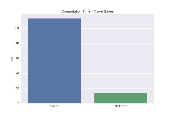
As you can see, the Naive Bayes classifier ran 8 times faster when operating on the sparse matrix!

from sklearn.linear_model import LogisticRegression
lr = LogisticRegression(random_state=99)
%timeit lr.fit(dataset, y)
%timeit lr.fit(sparse_dataset, y)

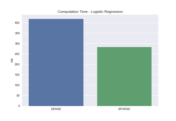
For logistic regression, we see roughly a 33% decrease in processing time. Not quite as performant as Naive Bayes but a big difference nonetheless.

from sklearn.svm import LinearSVC
svc = LinearSVC()
%timeit svc.fit(dataset, y)
%timeit svc.fit(sparse_dataset, y)

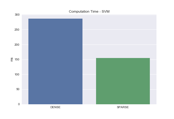
And finally, we have SVM. With sparse matrices we are able to achieve roughly a 50% reduction in processing time!

All in all, converting sparse matrices to the sparse matrix format almost always yields some efficiency in processing time. We saw this to be the case for Naive Bayes, Logistic Regression, and Support Vector Machines. Where do we not see improved processing times? Decision tree based algorithms like random forest.

How CSR Works

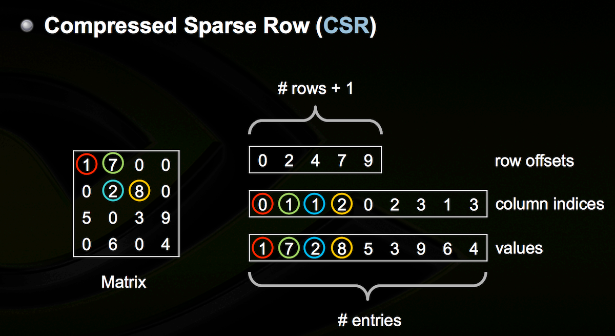Image Credit: Nathan Bell’s Sparse Matrix Representations & Iterative Solvers

CSR requires three arrays. The first array stores the cumulutive count of nonzero values in all current and previous rows. The second array stores column index values for each nonzero value. And the third array stores all nonzero values. I realize that may be confusing, so let’s walk through an example.

Refer to the diagram above. The first step is to populate the first array. It always starts with 0. Since there are two nonzero values in row 1, we update our array like so [0 2]. There are 2 nonzero values in row 2, so we update our array to [0 2 4]. Doing that for the remaining rows yields [0 2 4 7 9]. By the way, the length of this array should always be the number of rows + 1. Step two is populating the second array of column indices. Note that the columns are zero-indexed. The first value, 1, is in column 0. The second value, 7, is in column 1. The third value, 2, is in column 1. And so on. The result is the array [0 1 1 2 0 2 3 1 3]. Finally, we populate the third array which looks like this [1 7 2 8 5 3 9 6 4]. Again, we are only storing nonzero values.

Believe it or not, these three arrays allow us to perfectly reconstruct the original matrix. From here, common mathematical operations like addition or multiplication can be applied in an efficient manner. Note: the exact details of how the mathematical operations work on sparse matrix implementations are beyond the scope of this post. Suffice it to say there are many wonderful resources online if you are interested.

Summary

A matrix composed of many zeros is known as a sparse matrix. Sparse matrices have nice properties. How do you know if you have a sparse matrix? Use Matplotlib’s spy() method. Once you know your matrix is sparse, use Scipy’s CSR to convert its type from dense to sparse, check data compression, and apply any of the machine learning algorithms listed above.

In closing, I want you to leave you with this: if the original data matrix won’t fit into memory in the first place, can you think of a way to convert it to a sparse matrix anyway?

Stay tuned because I’ll answer that and many other questions in coming posts.

Additional Resources

Working with Sparse Matrices
Sparse Matrix Representations & Iterative Solvers
Scikit-learn Documentation
Scipy Sparse Matrices