
Model Tuning (Part 2 - Validation & Cross-Validation)

Introduction
Last time in Model Tuning (Part 1 - Train/Test Split) we discussed training error, test error, and train/test split. We learned that training a model on all the available data and then testing on that very same data is an awful way to build models because we have no indication as to how well that model will perform on unseen data. In other words, we don’t know if the model is essentially memorizing the data it’s seen or if it’s truly picking up the pattern inherent in the data (i.e. its ability to generalize).
To remedy that situation, we implemented train/test split that effectively holds some data aside from the model building process for testing at the very end when the model is fully trained. This allows us to see how the model performs on unseen data and gives us some indication as to whether the model generalizes or not.
Now that we have a solid foundation, we can move on to more advanced topics that will take our model-building skills to the next level. Specifically, we’ll dig in to the following topics:
- Bias-Variance Tradeoff
- Validation Set
- Model Tuning
- Cross-Validation
To make this concrete, we’ll combine theory and application. For the latter, we’ll leverage the Boston dataset in sklearn.
Please refer to the Boston dataset for details.
Our first step is to read in the data and prep it for modeling.
Get & Prep Data
Here’s a bit of code to get us going:
boston = load_boston()
data = boston.data
target = boston.target
And now let’s split the data into train/test split like so:
# train/test split
X_train, X_test, y_train, y_test = train_test_split(data,
                                                    target,
                                                    shuffle=True,
                                                    test_size=0.2,
                                                    random_state=15)
Setup
We know we’ll need to calculate training and test error, so let’s go ahead and create functions to do just that. Let’s include a meta-function that will generate a nice report for us while we’re at it. Also, Root Mean Squared Error (RMSE) will be our metric of choice.
def calc_train_error(X_train, y_train, model):
    '''returns in-sample error for already fit model.'''
    predictions = model.predict(X_train)
    mse = mean_squared_error(y_train, predictions)
    rmse = np.sqrt(mse)
    return mse

def calc_validation_error(X_test, y_test, model):
    '''returns out-of-sample error for already fit model.'''
    predictions = model.predict(X_test)
    mse = mean_squared_error(y_test, predictions)
    rmse = np.sqrt(mse)
    return mse

def calc_metrics(X_train, y_train, X_test, y_test, model):
    '''fits model and returns the RMSE for in-sample error and out-of-sample error'''
    model.fit(X_train, y_train)
    train_error = calc_train_error(X_train, y_train, model)
    validation_error = calc_validation_error(X_test, y_test, model)
    return train_error, validation_error
Time to dive into a little theory. Stay with it because we’ll come back around to the application side where you’ll see how all the pieces fit together.
Theory
Bias-Variance Tradeoff
Pay very close attention to this section. It is one of the most important concepts in all of machine learning. Understanding this concept will help you diagnose all types of models, be they linear regression, XGBoost, or Convolutional Neural Networks.
We already know how to calculate training error and test error. So far we’ve simply been using test error as a way to gauge how well our model will generalize. That was a good first step but it’s not good enough. We can do better. We can tune our model. Let’s drill down.
We can compare training error and something called validation error to figure out what’s going on with our model - more on validation error in a minute. Depending on the values of each, our model can be in one of three regions:
1) High Bias - underfitting
2) Goldilocks Zone - just right
3) High Variance - overfitting
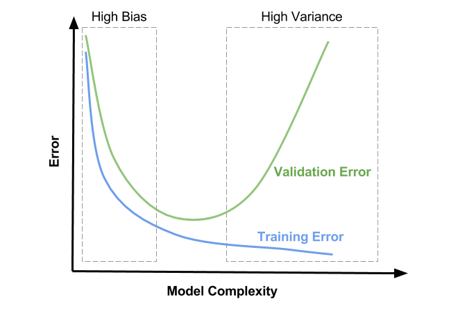
Plot Orientation
The x-axis represents model complexity. This has to do with how flexible your model is. Some things that add complexity to a model include: additional features, increasing polynomial terms, and increasing the depth for tree-based models. Keep in mind this is far from an exhaustive list but you should get the gist.
The y-axis indicates model error. It’s often measured as Mean-Squared Error (MSE) for Regression and Cross-Entropy or Accuracy for Classification.
The blue curve is Training Error. Notice that it only decreases. What should be painfully obvious is that adding model complexity leads to smaller and smaller training errors. That’s a key finding.
The green curve forms a U-shape. This curve represents Validation Error. Notice the trend. First it decreases, hits a minimum, and then increases. We’ll talk in more detail shortly about what exactly Validation Error is and how to calculate it.
High Bias
The rectangular box outlined by dashes to the left and labeled as High Bias is the first region of interest. Here you’ll notice Training Error and Validation Error are high. You’ll also notice that they are close to one another. This region is defined as the one where the model lacks the flexibility required to really pull out the inherent trend in the data. In machine learning speak, it is underfitting, meaning it’s doing a poor job all around and won’t generalize well. The model doesn’t even do well on the training set.
How do you fix this?
By adding model complexity of course. I’ll go into much more detail about what to do when you realize you’re under or overfitting in another post. For now, assuming you’re using linear regression, a good place to start is by adding additional features. The addition of parameters to your model grants it flexibility that can push your model into the Golidlocks Zone.
Goldilocks Zone
The middle region without dashes I’ve named the Goldilocks Zone. Your model has just the right amount of flexibility to pick up on the pattern inherent in the data but isn’t so flexible that it’s really just memorizing the training data. This region is marked by Training Error and Validation Error that are both low and close to one another. This is where your model should live.
High Variance
The dashed rectangular box to the right and labeled High Variance is the flip of the High Bias region. Here the model has so much flexiblity that it essentially starts to memorize the training data. Not surprisingly, that approach leads to low Training Error. But as was mentioned in the train/test post, a lookup table does not generalize, which is why we see high Validation Error in this region. You know you’re in this region when your Training Error is low but your Validation Error is high. Said another way, if there’s a sizeable delta between the two, you’re overfitting.
How do you fix this?
By decreasing model complexity. Again, I’ll go into much more detail in a separate post about what exactly to do. For now, consider applying regularization or dropping features.
Canonical Plot
Let’s look at one more plot to drive these ideas home.
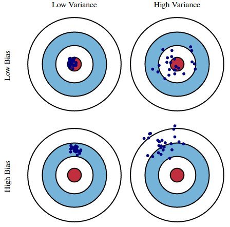
Imagine you’ve entered an archery competition. You receive a score based on which portion of the target you hit: 0 for the red circle (bullseye), 1 for the blue, and 2 for the while. The goal is to minimize your score and you do that by hitting as many bullseyes as possible.
The archery metaphor is a useful analog to explain what we’re trying to accomplish by building a model. Given different datasets (equivalent to different arrows), we want a model that predicts as closely as possible to observed data (aka targets).
The top Low Bias/Low Variance portion of the graph represents the ideal case. This is the Goldilocks Zone. Our model has extracted all the useful information and generalizes well. We know this because the model is accurate and exhibits little variance, even when predicting on unforeseen data. The model is highly tuned, much like an archer who can adjust to different wind speeds, distances, and lighting conditions.
The Low Bias/High Variance portion of the graph represents overfitting. Our model does well on the training data, but we see high variance for specific datasets. This is analagous to an archer who has trained under very stringent conditions - perhaps indoors where there is no wind, the distance is consistent, and the lighting is always the same. Any variation in any of those attributes throws off the archer’s accuracy. The archer lacks consistency.
The High Bias/Low Variance portion of the graph represents underfitting. Our model does poorly on any given dataset. In fact, it’s so bad that it does just about as poorly regardless of the data you feed it, hence the small variance. As an analog, consider an archer who has learned to fire with consistency but hasn’t learned to hit the target. This is analagous to a model that always predicts the average value of the training data’s target.
The High Bias/High Variance portion of the graph actually has no analog in machine learning that I’m aware of. There exists a tradeoff between bias and variance. Therefore, it’s not possible for both to be high.
Alright, let’s shift gears to see this in practice now that we’ve got the theory down.
Application
Let’s build a linear regression model of the Forest Fire dataset. We’ll investigate whether our model is underfitting, overfitting, or fitting just right. If it’s under or overfitting, we’ll look at one way we can correct that.
Time to build the model.
Note: I’ll use train_error to represent training error and test_error to represent validation error.
lr = LinearRegression(fit_intercept=True)

train_error, test_error = calc_metrics(X_train, y_train, X_test, y_test, lr)
train_error, test_error = round(train_error, 3), round(test_error, 3)

print('train error: {} | test error: {}'.format(train_error, test_error))
print('train/test: {}'.format(round(test_error/train_error, 1)))
The output looks like:
train error: 21.874 | test error: 23.817
train/test: 1.1
Hmm, our training error is somewhat lower than the test error. In fact, the test error is 1.1 times or 10% worse. It’s not a big difference but it’s worth investigating.
Which region does that put us in?
That’s right, it’s every so slightly in the High Variance region, which means our model is slightly overfitting. Again, that means our model has a tad too much complexity.
Unfortunately, we’re stuck at this point.
You’re probably thinking, “Hey wait, no we’re not. I can drop a feature or two and then recalculate training error and test error.”
My response is simply: NOPE. DON’T. PLEASE. EVER. FOR ANY REASON. PERIOD.
Why not?
Because if you do that then your test set is no longer a test set. You are using it to train your model. It’s the same as if you trained your model on the all the data from the beginning. Seriously, don’t do this. Unfortunately, practicing data scientists do this sometimes; it’s one of the worst things you can do. You’re almost guaranteed to produce a model that cannot generalize.
So what do we do?
We need to go back to the beginning. We need to split our data into three datasets: training, validation, test.
Remember, the test set is data you don’t touch until you’re happy with your model. The test set is used only ONE time to see how your model will generalize. That’s it.
Okay, let’s take a look at this thing called a Validation Set.
Validation Set
Three datasets from one seems like a lot of work but I promise it’s worth it. First, let’s see how to do this in practice.
# intermediate/test split (gives us test set)
X_intermediate, X_test, y_intermediate, y_test = train_test_split(data,
                                                                  target,
                                                                  shuffle=True,
                                                                  test_size=0.2,
                                                                  random_state=15)

# train/validation split (gives us train and validation sets)
X_train, X_validation, y_train, y_validation = train_test_split(X_intermediate,
                                                                y_intermediate,
                                                                shuffle=False,
                                                                test_size=0.25,
                                                                random_state=2018)
Now for a little cleanup and some output:
# delete intermediate variables
del X_intermediate, y_intermediate

# print proportions
print('train: {}% | validation: {}% | test {}%'.format(round(len(y_train)/len(target),2),
                                                       round(len(y_validation)/len(target),2),
                                                       round(len(y_test)/len(target),2)))
Which outputs:
train: 0.6% | validation: 0.2% | test 0.2%
If you’re a visual person, this is how our data has been segmented.
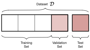
We have now three datasets depicted by the graphic above where the training set constitutes 60% of all data, the validation set 20%, and the test set 20%. Do notice that I haven’t changed the actual test set in any way. I used the same initial split and the same random state. That way we can compare the model we’re about to fit and tune to the linear regression model we built earlier.
Side note: there is no hard and fast rule about how to proportion your data. Just know that your model is limited in what it can learn if you limit the data you feed it. However, if your test set is too small, it won’t provide an accurate estimate as to how your model will perform. Cross-validation allows us to handle this situation with ease, but more on that later.
Time to fit and tune our model.
Model Tuning
We need to decrease complexity. One way to do this is by using regularization. I won’t go into the nitty gritty of how regularization works now because I’ll cover that in a future post. Just know that regularization is a form of constrained optimization that imposes limits on determining model parameters. It effectively allows me to add bias to a model that’s overfitting. I can control the amount of bias with a hyperparameter called lambda or alpha (you’ll see both, though sklearn uses alpha because lambda is a Python keyword) that defines regularization strength.
The code:
alphas = [0.001, 0.01, 0.1, 1, 10]
print('All errors are RMSE')
print('-'*76)
for alpha in alphas:
    # instantiate and fit model
    ridge = Ridge(alpha=alpha, fit_intercept=True, random_state=99)
    ridge.fit(X_train, y_train)
    # calculate errors
    new_train_error = mean_squared_error(y_train, ridge.predict(X_train))
    new_validation_error = mean_squared_error(y_validation, ridge.predict(X_validation))
    new_test_error = mean_squared_error(y_test, ridge.predict(X_test))
    # print errors as report
    print('alpha: {:7} | train error: {:5} | val error: {:6} | test error: {}'.
          format(alpha,
                 round(new_train_error,3),
                 round(new_validation_error,3),
                 round(new_test_error,3)))
And the output:
All errors are RMSE
----------------------------------------------------------------------------
alpha:   0.001 | train error: 22.93 | val error: 19.796 | test error: 23.959
alpha:    0.01 | train error: 22.93 | val error: 19.792 | test error: 23.944
alpha:     0.1 | train error: 22.945 | val error: 19.779 | test error: 23.818
alpha:       1 | train error: 23.324 | val error: 20.135 | test error: 23.522
alpha:      10 | train error: 24.214 | val error: 20.958 | test error: 23.356
There are a few key takeaways here. First, notice the U-shaped behavior exhibited by the validation error. It starts at 19.796, goes down for two steps and then back up. Also notice that validation error and test error tend to move together, but by no means is the relationship perfect. We see both errors decrease as alpha increases initially but then test error keeps going down while validation error rises again. It’s not perfect. It actually has a whole lot to do with the fact that we’re dealing with a very small dataset. Each sample represents a much larger proportion of the data than say if we had a dataset with a million or more records. Anyway, validation error is a good proxy for test error, especially as dataset size increases. With small to medium-sized datasets, we can do better by leveraging cross-validation. We’ll talk about that shortly.
Now that we’ve tuned our model, let’s fit a new ridge regression model on all data except the test data. Then we’ll check the test error and compare it to that of our original linear regression model with all features.
Setup Data, Model, & Calculate Errors
# train/test split
X_train, X_test, y_train, y_test = train_test_split(data,
                                                    target,
                                                    shuffle=True,
                                                    test_size=0.2,
                                                    random_state=15)

# instantiate model
ridge = Ridge(alpha=0.11, fit_intercept=True, random_state=99)

# fit and calculate errors
new_train_error, new_test_error = calc_metrics(X_train, y_train, X_test, y_test, ridge)
new_train_error, new_test_error = round(new_train_error, 3), round(new_test_error, 3)
Report Errors
print('ORIGINAL ERROR')
print('-' * 40)
print('train error: {} | test error: {}\n'.format(train_error, test_error))
print('ERROR w/REGULARIZATION')
print('-' * 40)
print('train error: {} | test error: {}'.format(new_train_error, new_test_error))
Here’s that output:
ORIGINAL ERROR
----------------------------------------
train error: 21.874 | test error: 23.817

ERROR w/REGULARIZATION
----------------------------------------
train error: 21.883 | test error: 23.673
A very small increase in training error coupled with a small decrease in test error. We’re definitely moving in the right direction. Perhaps not quite the magnitude of change we expected, but we’re simply trying to prove a point here. Remember this is a tiny dataset. Also remember I said we can do better by using something called Cross-Validation. Now’s the time to talk about that.
Cross-Validation
Let me say this upfront: this method works great on small to medium-sized datasets. This is absolutely not the kind of thing you’d want to try on a massive dataset (think tens or hundreds of millions of rows and/or columns). Alright, let’s dig in now that that’s out of the way.
As we saw in the post about train/test split, how you split smaller datasets makes a significant difference; the results can vary tremendously. As the random state is not a hyperparameter (seriously, please don’t do that), we need a way to extract every last bit of signal from the data that we possibly can. So instead of just one train/validation split, let’s do K of them.
This technique is appropriately named K-fold cross-validation. Again, K represents how many train/validation splits you need. There’s no hard and fast rule about how to choose K but there are better and worse choices. As the size of your dataset grows, you can get away with smaller values for K, like 3 or 5. When your dataset is small, it’s common to select a larger number like 10. Again, these are just rules of thumb.
Here’s the general idea for 10-fold CV:
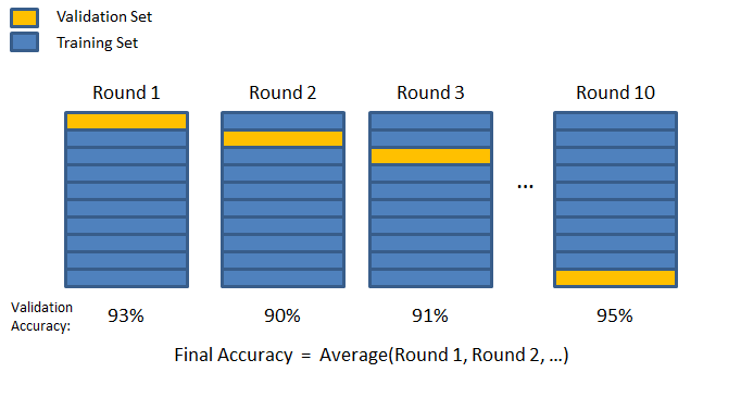
You segment off a percentage of your training data as a validation fold.
Technical note: Be careful with terminology. Some people will refer to the validation fold as the test fold. Unfortunately, they use the terms interchangeably, which is confusing and therefore not correct. Don’t do that. The test set is the pure data that only gets consumed at the end, if it exists at all.
Once data has been segmented off in the validation fold, you fit a fresh model on the remaining training data. Ideally, you calculate train and validation error. Some people only look at validation error, however.
The data included in the first validation fold will never be part of a validation fold again. A new validation fold is created, segmenting off the same percentage of data as in the first iteration. Then the process repeats - fit a fresh model, calculate key metrics, and iterate. The algorithm concludes when this process has happened K times. Therefore, you end up with K estimates of the validation error, having visited all the data points in the validation set once and numerous times in training sets. The last step is to average the validation errors for regression. This gives a good estimate as to how well a particular model will perform.
Again, this method is invaluable for tuning hyperparameters on small to medium-sized datasets. You technically don’t even need a test set. That’s great if you just don’t have the data. For large datasets, use a simple train/validation/test split strategy and tune your hyperparameters like we did in the previous section.
Alright, let’s see K-fold CV in action.
Sklearn & CV
There’s two ways to do this in sklearn, pending what you want to get out of it.
The first method I’ll show you is cross_val_score, which works beautifully if all you care about is validation error.
The second method is KFold, which is perfect if you require train and validation errors.
Let’s try a new model called LASSO just to keep things interesting.
cross_val_score
from sklearn.model_selection import cross_val_score

alphas = [1e-4, 1e-3, 1e-2, 1e-1, 1, 1e1]

val_errors = []
for alpha in alphas:
    lasso = Lasso(alpha=alpha, fit_intercept=True, random_state=77)
    errors = np.sum(-cross_val_score(lasso,
                                     data,
                                     y=target,
                                     scoring='neg_mean_squared_error',
                                     cv=10,
                                     n_jobs=-1))
    val_errors.append(np.sqrt(errors))
Let’s checkout the validation errors associated with each alpha.
# RMSE
print(val_errors)
Which returns:
[18.64401379981868, 18.636528438323769, 18.578057471596566, 18.503285318281634, 18.565586130742307, 21.412874355105991]
Which value of alpha gave us the smallest validation error?
print('best alpha: {}'.format(alphas[np.argmin(val_errors)]))
Which returns: best alpha: 0.1
K-Fold
from sklearn.model_selection import KFold

K = 10
kf = KFold(n_splits=K, shuffle=True, random_state=42)

for alpha in alphas:
    train_errors = []
    validation_errors = []
    for train_index, val_index in kf.split(data, target):

        # split data
        X_train, X_val = data[train_index], data[val_index]
        y_train, y_val = target[train_index], target[val_index]

        # instantiate model
        lasso = Lasso(alpha=alpha, fit_intercept=True, random_state=77)

        #calculate errors
        train_error, val_error = calc_metrics(X_train, y_train, X_val, y_val, lasso)

        # append to appropriate list
        train_errors.append(train_error)
        validation_errors.append(val_error)

    # generate report
    print('alpha: {:6} | mean(train_error): {:7} | mean(val_error): {}'.
          format(alpha,
                 round(np.mean(train_errors),4),
                 round(np.mean(validation_errors),4)))
Here’s that output:
alpha: 0.0001 | mean(train_error): 21.8217 | mean(val_error): 23.3633
alpha:  0.001 | mean(train_error): 21.8221 | mean(val_error): 23.3647
alpha:   0.01 | mean(train_error): 21.8583 | mean(val_error): 23.4126
alpha:    0.1 | mean(train_error): 22.9727 | mean(val_error): 24.6014
alpha:      1 | mean(train_error): 26.7371 | mean(val_error): 28.236
alpha:   10.0 | mean(train_error):  40.183 | mean(val_error): 40.9859
Comparing the output of cross_val_score to that of KFold, we can see that the general trend holds - an alpha of 10 results in the largest validation error. You may wonder why we get different values. The reason is that the data was split differently. We can control the splitting procedure with KFold but not cross_val_score. Therefore, there’s no way I know of to perfectly sync the two procedures without an exhaustive search of splits or writing the algorithm from scratch ourselves. The important thing is that each gives us a viable method to calculate whatever we need, whether it be purely validation error or a combination of training and validation error.
Update: sklearn has a method called cross_validate that will capture training and validation errors for you. It’ll even spit out how long it took to train a model for each fold as well as the time it took to score the model on each validation set.
Wrap Up
Once you’ve tuned your hyperparameters, what do you do? Simply train a fresh model on all the data so you can extract as much information as possible. That way your model will have the best predictive power on future data. Mission complete!
Summary
We discussed the Bias-Variance Tradeoff where a high bias model is one that is underfit while a high variance model is one that is overfit. We also learned that we can split data into three groups for tuning purposes. Specifically, the three groups are train, validation, and test. Remember the test set is used only one time to check how well a model generalizes on data it’s never seen. This three-group split works exceedingly well for large datasets but not for small to medium-sized datasets, though. In that case, use cross-validation (CV). CV can help you tune your models and extract as much signal as possible from the small data sample. Remember, with CV you don’t need a test set. By using a K-fold approach, you get the equivalent of K-test sets by which to check validation error. This helps you diagnose where you’re at in the bias-variance regime.