Introduction to Time Series

Introduction

Dealing with data that is sequential in nature requires special techniques. Unlike traditional Ordinary Least Squares or Decision Trees where the observations are independent, time series data is such that there is correlation between successive samples. In other words, order very much matters. Think stock prices or daily temperatures. Identifying time series data and knowing what to do next is a valuable skill for any modeler.

The first step on our journey is to identify the three components of time series data:

1. Trend
2. Seasonality
3. Residuals

Trend, as its name suggests, is the overall direction of the data. Seasonality is a periodic component. And the residual is what’s left over when the trend and seasonality have been removed. Residuals are random fluctuations. You can think of them as a noise component.

Let’s look at a few plots to make sure we understand trend, seasonality, and residuals.

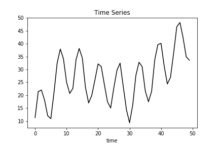
Time Series Data

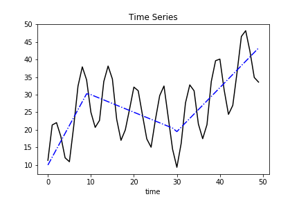
Trend

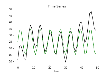
Seasonality

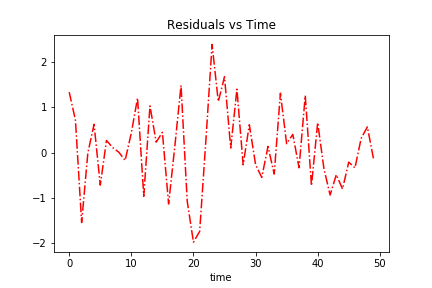
Residuals

Now that you have the big picture, let’s look at the nuts and bolts. I’ll show you how I created the data above, how to create derivatives of the plots shown above, and how to decompose a time series model in Python.

Create Time Series Data

Time series data is data that is measured at equally-spaced intervals. Think of a sensor that takes measurements every minute.

A sensor that takes measurements at random times is not time series.

Trend

The first step is to create a time interval with equal spacing.

import numpy as np
time = np.arange(50)

Great. Now to construct the trend.

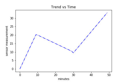
Sticking with the sensor example, suppose the sensor is oriented towards an oscillating fan that alternates right and left. The trend component captures the wind speed as someone adjusts the fan speed. Increased fan speed translates to increased sensor measurements.

trend = np.empty_like(time, dtype='float')
for t in time:
    if t < 10:
        trend[t] = t * 2.25 
    elif t < 30:
        trend[t] = t * -0.5 + 25
    else:
        trend[t] = t * 1.25 - 28

Better plot it.

import matplotlib.pyplot as plt
plt.plot(time, trend, 'b.')
plt.title("Trend vs Time")
plt.xlabel("minutes")
plt.ylabel("sensor measurement")

Here’s the result:

Seasonality

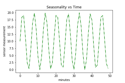
The next step is to create a periodic element. The wind speed sensor analog is the wind speed that’s captured as the fan sweeps left to right and back again.

Here’s an example of how we can create that:

seasonal = 10 + np.sin(time) * 10

Notice how both trend and seasonality are a function of time but independent of one another.

Also, here’s a plot of the seasonality component:

plt.plot(time, seasonal, 'g-.')
plt.title("Seasonality vs Time")
plt.xlabel("minutes")
plt.ylabel("sensor measurement")

Residual

The last component is the residual. This is a noise component, as mentioned earlier. We can fabricate that like so:

np.random.seed(10)  ## reproducible results
residual = np.random.normal(loc=0.0, scale=1, size=len(time))

And the plot:

plt.plot(time, residual, 'r-.')
plt.title("Residuals vs Time")
plt.xlabel("minutes")
plt.ylabel("electricity demand")

Aggregating Components

Now comes time to aggregate the three components: trend, seasonality, and residuals. This will give us the time series data were looking for.

As it turns out, there are two major ways to aggregate (or decompose, as we’ll see later) time series data.

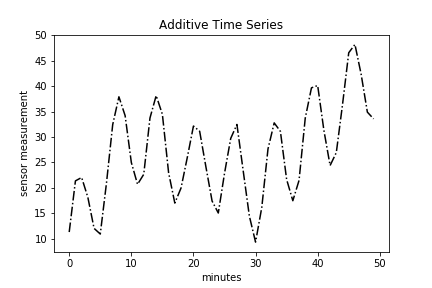
Additive

The first way is simply a sum of the three components.

That’s as easy as additive = trend + seasonal + residual.

The corresponding plot is:

plt.plot(time, additive, 'k-.')
plt.title("Additive Time Series")
plt.xlabel("minutes")
plt.ylabel("sensor measurement");

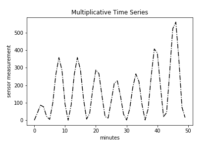
Multiplicative

The second way to decompose time series data is a multiplication of all three components.

We can stitch that together with:

# ignore residual to make pattern obvious
ignored_residual = np.ones_like(residual)
multiplicative = trend * seasonal * ignored_residual

The corresponding plot is:

plt.plot(time, multiplicative, 'k-.')
plt.title("Multiplicative Time Series")
plt.xlabel("minutes")
plt.ylabel("sensor measurement")

Additive vs Multiplicative?

The primary question likely bouncing around your head is how can I tell if a time series is additive or multiplicative? Simply plotting the original time series data, called a run-sequence plot, is one way to do so. If the seasonality and residual components are independent of the trend, then you have an additive series. If the seasonality and residual components are in fact dependent, meaning they fluctuate on trend, then you have a multiplicative series. Look at the additive and multiplicative plots above. You’ll notice a big difference in the amplitudes of the peaks and troughs. Specifically, the amplitude of the seasonal component of the multiplicative time series is changes with trend.

Time Series Decomposition with Python

You’ll likely never know how real-world data was generated. However, I’m about to show you a powerful tool that will allow you to decompose a time series into its components. Let’s see how simple it is.

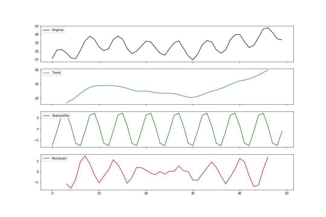
Additive Decomposition

from statsmodels.tsa.seasonal import seasonal_decompose
ss_decomposition = seasonal_decompose(x=additive, 
                                      model='additive', 
                                      freq=6)
estimated_trend = ss_decomposition.trend
estimated_seasonal = ss_decomposition.seasonal
estimated_residual = ss_decomposition.resid

Note that you must provide the frequency. We can see from the additive and multiplicative plots that the frequency is about 6. There are more sophisticated ways to determine this number empirically, but that’s for another tutorial. Let’s keep things simple for now.

Now that we have the pieces let’s put them all together.

fig, axes = plt.subplots(4, 1, sharex=True, sharey=False)
fig.set_figheight(10)
fig.set_figwidth(15)

axes[0].plot(additive, 'k', label='Original')
axes[0].legend(loc='upper left');

axes[1].plot(estimated_trend, label='Trend')
axes[1].legend(loc='upper left');

axes[2].plot(estimated_seasonal, 'g', label='Seasonality')
axes[2].legend(loc='upper left');

axes[3].plot(estimated_residual, 'r', label='Residuals')
axes[3].legend(loc='upper left')

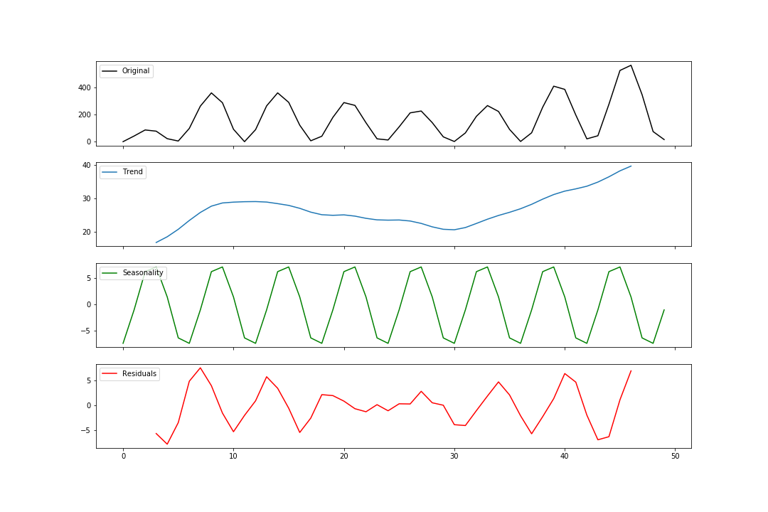
Multiplicative Decomposition

Multiplicative decomposition follows the exact same pattern. The only major change is that we change model to ‘multiplicative’.

ss_decomposition = seasonal_decompose(x=multiplicative, 
                                      model='multiplicative', 
                                      freq=6)
estimated_trend = ss_decomposition.trend
estimated_seasonal = ss_decomposition.seasonal
estimated_residual = ss_decomposition.resid

Some more matplotlib code:

fig, axes = plt.subplots(4, 1, sharex=True, sharey=False)
fig.set_figheight(10)
fig.set_figwidth(15)

axes[0].plot(multiplicative, label='Original')
axes[0].legend(loc='upper left')

axes[1].plot(estimated_trend, label='Trend')
axes[1].legend(loc='upper left')

axes[2].plot(estimated_seasonal, label='Seasonality')
axes[2].legend(loc='upper left')

axes[3].plot(estimated_residual, label='Residuals')
axes[3].legend(loc='upper left')

Viola! We have a multiplicative decomposition.

---

Summary

In this tutorial you should have learned:

1. Time series data is composed of three components: trend, seasonality, residual
2. Time series can be additive or multiplicative
3. How to decompose a time series model with Python