
Linear Regression 101 (Part 1 - Basics)

Introduction
Pretend you’re a pediatrician and that your pint-sized patients come in for monthly checkups starting at birth. Thankfully, you’ve kept a log of each baby’s weight at each checkup for the first 12 months. You’ve accumulated a good bit of data that looks like this:
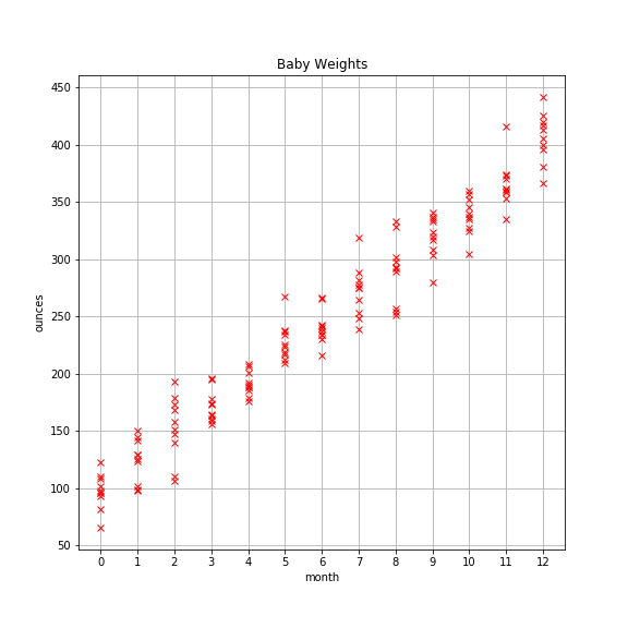
There appears to be a strong linear pattern here. It’d be nice if you could create a model that captures that pattern. That way you could use it as a means to compare new patients to see how they’re progressing, and if there are any abnormalities in weight (over or under) that you should be concerned about.
But how to build the model?
With linear regression of course!
Overview
Linear regression is simple yet surprisingly powerful. In this simple case, we have a single predictor variable (aka feature) called month. Linear regression with a single variable or feature is called univariate linear regression. The output of linear regression is an estimate of the outcome variable (aka target), which in this case is a baby’s weight in ounces.
The equation of our model looks like this:
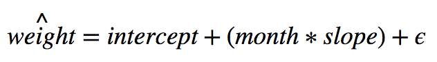
Notice the hat on weight. This signifies that our model creates an estimate of the target variable. It is not the actual value for a given baby. It’s important to remember that.
The intercept is the expected value of a newborn. This is the same as saying a baby at month 0 is expected to weigh the value of the intercept. Another way to think about it is by looking at the equation of the model. The slope is nonzero. We can see that in the graph above. Therefore, when month is 0, the intercept is the model’s estimate for a baby’s weight at birth because 0 times slope equals 0 which leaves us with the intercept and another term we’ll get to shortly.
For nonbirth weights, we simply sum the intercept with the product of month and slope.
You may be wondering about that funny looking e called epsilon. That signifies error. Error comes in two flavors: reducible and irreducible. Reducible error is error that results when your model is not extracting all the structure or pattern in the data. Irreducible error is what’s left over. For nontrivial datasets, there will always be irreducible error, so don’t expect to create a model that perfectly predicts every example.
Side note: it’s important to keep in mind that a model is an approximation of reality. Rarely if ever does a model take all factors into account. In the case of babies, we’re using age in months as a way to estimate a baby’s weight in ounces. Obviously, genetics and environmental factors play a major role in a baby’s weight, but using age in months is a great proxy in this case.
At this point you should have a burning question zipping around in your brain: just how the heck do we find values for the intercept and slope?
The short answer is there are two ways. There is an analytical solution. This means there is an exact solution like solving 2x=6. There is also a numerical approximation method known as Gradient Descent.
Now you’re likely wondering why anyone would choose to use a numerical approximation method like Gradient Descent when there exists an exact solution, but it turns out there is good reason for this.
If your data is relatively small, meaning it will fit in memory, then the analytical solution is your best bet. If, however, your data is large and will not fit in memory, you’re stuck unless you use a numerical approach like Gradient Descent.
I won’t go into any more detail on Gradient Descent here as that will be a discussion for another post. However, with the foundation of knowledge we have now, we can discuss how to find the intercept and slope terms.
Terminology
It’s time to get more formal.
Let X signify the data in matrix form. Unsurprisingly, it is known as the data matrix.
Let y signify observed values in vector form. It is known as the target (aka the thing we’re trying to predict).
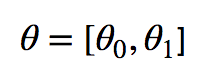
The intercept and slope are known as parameters or coefficients. You will often see them labeled as beta or theta. The machine learning literature tends to use thetas so that’s what I’m partial to. Hence, I will use thetas from here on out. Just know that statistians and others use betas in the same way.
We can create a vector of thetas like so:
Finding Parameters
The analytical solution to finding the values of the parameters is straight forward.
The equation is:
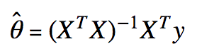
I’m assuming you’re comfortable with linear algebra. If you’re unfamiliar with vector or matrix transposes, vector or matrix multiplication, or matrix inverses, please review those topics separately.
Now let’s write some Python code to find the parameters using a little bit of NumPy.
First, I’ll show you how I generated the data in the very first plot of this post:
import numpy as np

# reproducibility
np.random.seed(10)

# generate data
babies = range(10)
months = np.arange(13)
data = [(month, np.dot(month, 24.7) + 96 + np.random.normal(loc=0, scale=20))
        for month in months
        for baby in babies]
month_data = [element[0] for element in data]
weight_data = [element[1] for element in data]
Then we’ll need to transform the data so it’s in the proper format.
X = np.array(month_data)
X = np.c_[np.ones(X.shape[0]), X] # little trick to add vector of 1's
y = np.array(weight_data)
Technical note: I add the vector of ones so we can find the intercept. Without this step, only the parameters associated with the features are returned. Think of it as the intercept coefficient times 1. The vector of ones acts like a fake feature, in other words. It’s really just a simple linear algebra trick.
Next, let’s create a function to find the parameters. Pay special attention because this is the key bit of code; this is where the magic happens.
def ols(X, y):
    '''returns parameters based on Ordinary Least Squares.'''
    xtx = np.dot(X.T, X) ## x-transpose times x
    inv_xtx = np.linalg.inv(xtx) ## inverse of x-transpose times x
    xty = np.dot(X.T, y) ## x-transpose times y
    return np.dot(inv_xtx, xty)
Finally, let’s push the observational data through the function to find the thetas.
# find parameters
params = ols(X,y)
print('intercept: {} | slope: {}'.format(params[0], params[1]))
The result looks like this: intercept: 97.94349022705887 | slope: 24.680165065438715
Now’s as a good a time as any to plot the regression line over our data to see how we did.
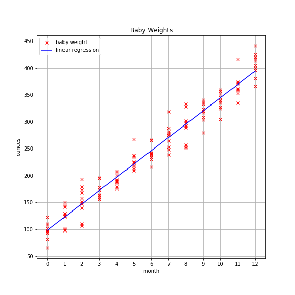
Looks pretty good!
Multivariate Linear Regression
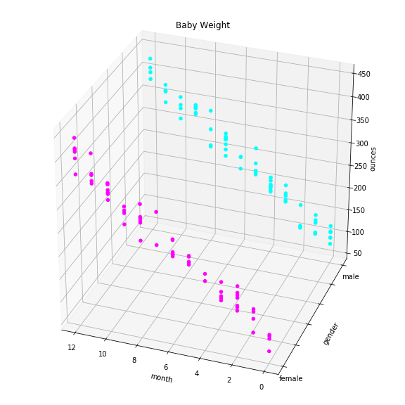
Now we’re ready to tackle more interesting problems. Suppose you were keeping track not only of which month you collected weights but also the gender of the child. So for each monthly checkup, you have month, gender, and weight. In this case, month and gender are features and weight is still the target.
The beautiful thing is that all the hard work we’ve done thus far transfers over seamlessly. We can solve this problem. We simply need to add an additional parameter for each new feature. Hooray!
Let’s add a feature called gender and update our data matrix X.
gender = np.random.binomial(n=1, p=0.5, size=len(babies)*len(months)) ## male=0, female=1
X = np.c_[X, gender]
Here’s the plot:
Instead of finding a best fitting line of the data, we’re looking for the best fitting plane. We solve the same way. Watch this.
multivariate_params = ols(X,y)
print(multivariate_params)
The output is: [ 95.46395681 24.63320421 5.6979177 ]
Final plot:
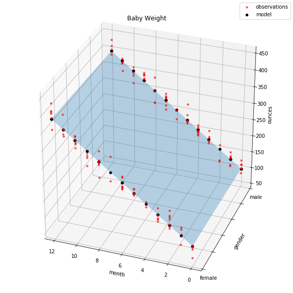
The red dots indicate actual observations of baby weights. The light blue plane shows the solution space of our model. Actually, that’s not entirely true. If we swapped the indicator feature gender with a continuous one, the plane would indeed represent the full range of solutions. However, because gender can only take values 0 or 1, our solution ends up being two lines, subsets of the plane, indicated by the black dots.
Where To Go From Here?
We talked about linear regression terminology and how to find its model parameters, at least analytically. What we haven’t talked about yet is metrics, model assumptions, potential pitfalls, and how to handle them. We’ll pick up next time with metrics so stay tuned!