
Linear Regression 101 (Part 2 - Metrics)
Introduction
We left off last time (Part 1) discussing the basics of linear regression. Specifically, we learned key terminology and how to find parameters for both univariate and multivariate linear regression. Now we’ll turn our focus to metrics pertaining to our model.
We’ll look at the following key metrics:
- Sum of Squared Errors (SSE)
- Total Sum of Squares (SST)
- R^2
- Adjusted R^2
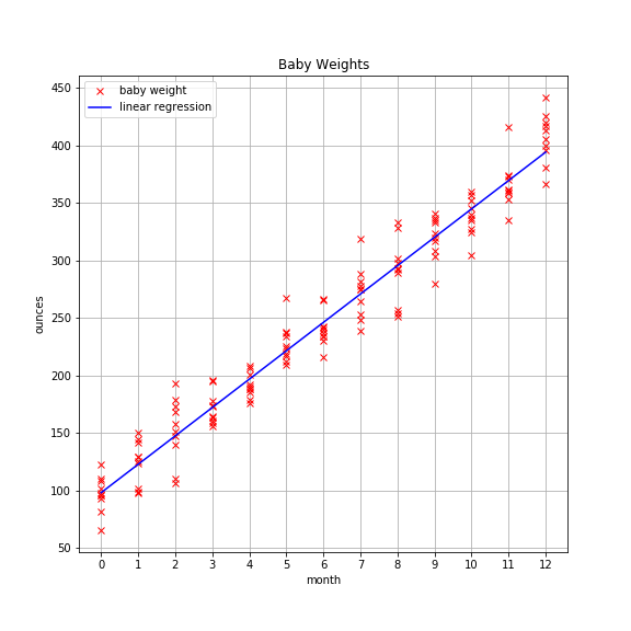
To keep things simple, we’ll use the univariate baby weight data from the previous post and leverage sklearn to find the model parameters.
Here’s how I generated the data again:
import numpy as np

# reproducibility
np.random.seed(10)

# generate data
babies = range(10)
months = np.arange(13)
data = [(month, np.dot(month, 24.7) + 96 + np.random.normal(loc=0, scale=20))
        for month in months
        for baby in babies]
month_data = [element[0] for element in data]
weight_data = [element[1] for element in data]
Let’s fit the model. Instead of using the linear algebra code from the first post, we can use the scikit-learn (sklearn) module to do the heavy lifting for us. Here’s how you do that:
from sklearn.linear_model import LinearRegression

X = np.array(month_data).reshape(-1,1)
y = weight_data

lr = LinearRegression(fit_intercept=True)
lr.fit(X, y)
Technical note: X contains .reshape(-1,1) which creates a fake 2D array for fitting. This trick pops up quite frequently so you should remember it.
As a reminder, the plot looks like this:
Metrics To Assess Model
We will investigate four key metrics:
- Sum of Squared Errors (SSE)
- Total Sum of Squares (SST)
- R^2
- Adjusted R^2
First, the formulas:
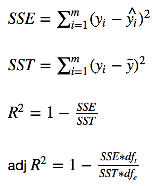
Keep in mind that y_i is the observed target value, y-hat_i is the predicted value, and y-bar is the mean value. Here, m represents the total number of observations. For example, if there are 25 baby weigths, then m equals 25.
Lastly, df_t is the degrees of freedom of the estimate of the population variance of the dependent variable and df_e is the degrees of freedom of the estimate of the underlying population error variance. If df_t and df_e don’t make much sense, don’t worry about it. They’re simply used to calculate adjusted R^2.
I’m going to assume you’re familiar with basic OOP. If not, you should still get the main idea, though some nuances may be lost.
Without further ado, let’s create a class to capture the four key statistics about our data.
class Stats:

    def __init__(self, X, y, model):
        self.data = X
        self.target = y
        self.model = model
        ## degrees of freedom population dep. variable variance
        self._dft = X.shape[0] - 1
        ## degrees of freedom population error variance
        self._dfe = X.shape[0] - X.shape[1] - 1

    def sse(self):
        '''returns sum of squared errors (model vs actual)'''
        squared_errors = (self.target - self.model.predict(self.data)) ** 2
        return np.sum(squared_errors)

    def sst(self):
        '''returns total sum of squared errors (actual vs avg(actual))'''
        avg_y = np.mean(self.target)
        squared_errors = (self.target - avg_y) ** 2
        return np.sum(squared_errors)

    def r_squared(self):
        '''returns calculated value of r^2'''
        return 1 - self.sse()/self.sst()

    def adj_r_squared(self):
        '''returns calculated value of adjusted r^2'''
        return 1 - (self.sse()/self._dfe) / (self.sst()/self._dft)
While we’re at it, let’s create a pretty print function to generate a nice looking report.
def pretty_print_stats(stats_obj):
    '''returns report of statistics for a given model object'''
    items = ( ('sse:', stats_obj.sse()), ('sst:', stats_obj.sst()),
             ('r^2:', stats_obj.r_squared()), ('adj_r^2:', stats_obj.adj_r_squared()) )
    for item in items:
        print('{0:8} {1:.4f}'.format(item[0], item[1]))
Now the report.
stats = Stats(X, y, lr)
pretty_print_stats(stats)
And the output:
sse:     50253.0180
sst:     1158834.2148
r^2:     0.9566
adj_r^2: 0.9563
Interpretation
(SSE)
SSE is measure of how far off our model’s predictions are from the observed values. A value of 0 indicates that all predications are spot on. A non-zero value indicates errors. We expect a non-zero value. Why? Because there is always irreducible error that we just can’t get around, unless we’re dealing with some trivial problem.
Keep in mind the errors are squared.
Why is that?
Answer: squaring the values makes them all positive. If we didn’t square them, then we’d have some positive and some negative values. No matter how you slice it, you end up with error that looks smaller than it is in reality.
But why not use absolute error instead of squared error?
If you think about what squaring does to large numbers, you’ll realize that we’re really penalizing large errors. It’s like saying, it’s okay to miss on the close points but don’t allow large deviations between the model and the most distant points. This makes sense for some datasets but not others.
Consider the converse, though. There’s a data point or points that deviate from the general trend, causing large squared errors. These anomalous data points are often called outliers, and they can wreak havoc on the performance of your model. Much more on this in the next post.
(SST)
SST is a measure of the variance in the target variable. It is measured simply as the sum of the squared difference between each observation and the target mean.
(R^2)
R^2 measures how much variance is captured by the model. The range for Ordinary Least Squares is [0,1]. It is possible to get negative values for R^2 but that would require a fitting procedure other than OLS or non-linear data. Always know your assumptions!
(Adjusted R^2)
Adjusted R^2 is the same as standard R^2 except that it penalizes models when additional features are added. This naturally leads to the next section about why R^2 is a poor metric to use.
Why R^2 is a Poor Metric
R^2 will only go up as additional features are added, even if those features provide the model no new predictive power. See the example below.
Generate Dummy Data
def generate_random_data(num_rows, num_features, random_state=None):
    '''returns 2D numpy array based on user-defined inputs with random features.'''
    if random_state:
        np.random.seed(random_state)
    for feature in range(num_features):
        if feature == 0:
            data = np.random.uniform(size=num_rows)
        elif feature == 1:
            data = np.hstack((data.reshape(-1,1),
                              np.random.uniform(size=num_rows).reshape(-1,1)))
        else:
            data = np.hstack((data, np.random.uniform(size=num_rows).reshape(-1,1)))
    return data
Compare R^2 and Adjusted R^2
min_features = 1
max_features = 100

r_squared = []
adj_r_squared = []

y = generate_random_data(num_rows=200, num_features=1, random_state=99)

for features in range(min_features, max_features+1):
    X = generate_random_data(num_rows=200, num_features=features, random_state=101)
    results = sm.OLS(y, X).fit()
    r_squared.append(results.rsquared)
    adj_r_squared.append(results.rsquared_adj)
Plot Varying Number of Features
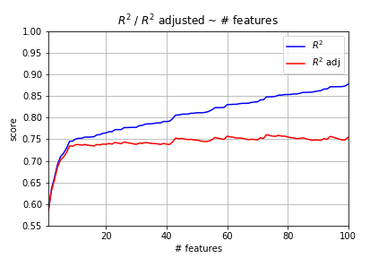
Ouch! That’s bad news. We generated random data. There’s absolutely no reason why including more features should lead to a better model. Yet, it’s clear from the plot above that R^2 only increases under these conditions. However, adjusted R^2 levels out because of the penalty involved.
The big takeaway here is that you cannot compare two linear regression models with differing numbers of features using R^2 alone. It just cannot be done. Adjusted R^2 works, though.
Wrap Up
As we’ll see in a future post, there are better ways to assess machine learning models, namely in-sample vs out-of-sample metrics and cross-validation. More on those in a future post about train/test split and cross-validation.
Next time we’ll dive into linear regression assumptions, pitfalls, and ways to address problems.